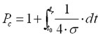
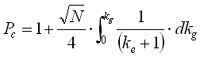
Abstract A convenient measure for the determination of the quality of a gradient separation is the peak capacity Pc (also sometimes abbreviated as nc). It is defined as the number of peaks that can be put into the gradient time frame with a defined resolution.
LevelAdvanced
Commonly, one uses a value of 4 times the standard deviation σ of a peak for peak spacing.
 (9)
(9)
The value of 1 stems from the fact that one will have at least one peak, i.e. the unretained peak.
We can use a simple procedure for the estimate of the peak capacity in a gradient chromatogram. Assuming that peaks elute until the end of the gradient, we can simply measure the peak width w for a number n of peaks that are well spaced over the chromatogram and use the following equation: 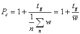 (10a)
(10a)
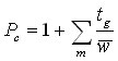
In other words, we divide the gradient run time by the average peak width . If the peaks do not elute over the entire gradient run time, we use the time to the elution of the last peak. If we have a segmented gradient or other forms of a gradient where the peak width changes significantly with the gradient run time, the peak capacity should be calculated by adding up the contributions for each segment m:
 (10b)
(10b)
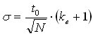
For a theoretical evaluation of the peak capacity, we need to replace the standard deviation in equation 9 with an expression that describes the change of the peak width with the evolution of the gradient. The standard deviation of every peak depends on the plate count N and on the retention factor at the point of elution ke:
 (11)
(11)
Combining equations 9 and 11 and using the gradient retention factor kg, we obtain:  (12)
(12)
Here we have made the assumption that the plate count is the same for all analytes. This equation can be solved for a range of cases. The simplest situation is the one where the peak width is assumed to remain constant. This is the case for typical reversed-phase peptide separations [4], or for very steep gradient separations as used in MS supported fast reversed-phase gradient separations [5]. Then, the peak capacity for the entire gradient can simply be expressed as:
 (13)
(13)
and the denominator contains the terms for the execution of the gradient. One can learn that for a steep gradient with a large G the peak capacity is smaller than for a flat gradient with a small G, where the peak capacity approaches a constant value.
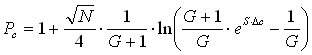
For small molecules in a more realistic gradient, the solution of the equation becomes a bit more complex [3]:
 (14)
(14)
This form of the equation can be used to judge the peak capacity for gradients with a fixed composition. If, on the other hand, we are interested in the analysis to a fixed last eluting analyte, the equation becomes simpler. Recognizing from equation 3b that ![]() , we substitute equation 2 into equation 14 and obtain:
, we substitute equation 2 into equation 14 and obtain:
![]() (15)
(15)
k0 is the retention factor of the last eluting analyte at the beginning of the gradient. This equation just describes a different analytical problem, and we can refer to it as the peak capacity to the last analyte.
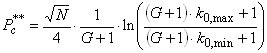
Lloyd Snyder had created another scenario [6] for examining the peak capacity of a separation. He formulated the concept of the sample peak capacity P**, which is defined as the number of peaks that fit into the separation space between the first and the last peak. The value can be obtained readily by subtracting the peak capacity from equation 15 for the first peak in the chromatogram (k0,min) from the same value for the last peak in the chromatogram (k0,max). As previously, we assume that G is constant, and we obtain:
 (16)
(16)
For a sufficiently large retention factor k0,min, this can be simplified further: 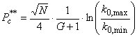 (17)
(17)
Once again, we can compare this equation to the well known resolution equation, equation 5. One can clearly see the similarities, especially if G is abbreviated (as above for equation 8) with the retention factor at the point of elution ke:
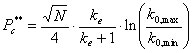 (18)
(18)
The plate count affects gradient separations and isocratic separations equally. The function in the retention factor is identical to the same function for the resolution equation (equations 5 and 8). We see that a higher retention factor at the point of elution leads to a better peak capacity in gradients, just as a higher isocratic retention factor leads to higher resolution. The last factor is a representation of the chemistry of the separation, i.e. the α-value for isocratic chromatography or the separation space in gradient chromatography. It is pleasing to see, how equations similar to the old-fashioned resolution equation (equation 5) emerge in different circumstances in gradient chromatography.
In chromatography, we would like to improve the overall resolution in the chromatogram, preferentially without having to increase the analysis time. Equations 8 and 18 show us how to do this. We can increase ke by flattening the gradient, and we can flatten the gradient at an equal run time by increasing the flow rate. As we increase the flow rate, the plate count decreases. Thus there is a compromise for every analysis between the gain in resolution by the expansion of the gradient and the reduction in resolution due to the loss in plates. This can be treated mathematically for multiple cases of general interest [4, 5], and I will discuss two cases in more detail in the following sections.
Case 1: Peak capacity for generic analyses
In the world of combinatorial synthesis, the product analysis can in general not be optimized for every synthesis, and a generic method is preferred. In the case of a peptide analysis of a protein hydrolysate, one often starts similarly with a generic analytical protocol for the elution of all peptides. In the case of the analysis of a drug in rat or mouse plasma, one also often prefers a standard analytical protocol, rather than a specific protocol for the drug that has been administered. In all these cases, one would like to establish a well optimized method that provides maximum resolution, often maximum resolution within a given analysis time.
For such an optimization, we can examine equation 14, or the more simplified equation 13. We know the solvent range, in which our compounds of interest are eluting. Therefore the change in the solvent composition ∆c is defined. The coefficient S is defined by the type of analytes that we are dealing with. In order to maximize the peak capacity in either equation 13 or 14, we can change the plate count N or the gradient slope G. For a given column and a given gradient run time, both can be changed simultaneously when we change t0. Thus there is the desire to find the best t0, i.e. the best velocity, for maximizing the peak capacity, for a given gradient run time. While equation 14 is general, we need to preselect a few parameters, including the column, for doing this type of analysis. This is done in Figure 4 for a 15 cm 3.9 mm i.d. 5 μm column for an analysis of low molecular weight samples at 30 °C for a gradient from 5% to 95% organic.
We can see that the peak capacity increases with the gradient run time. At the same time we observe that there is a flow rate optimum for every run time. For the 5 μm column, the optimum for the 512-minute (~8.5 hours) gradient is at a very slow flow rate, around 0.3 mL/min. On the other hand, for the 8-minute gradient, the preferred flow rate is around 3 mL/min. For a 1-hour gradient, the optimum flow rate is found around 1 mL/min, in agreement with the practical experience.
The second diagram in Figure 4 shows the improvement that one will get from a shorter 10 cm column packed with smaller particles. At long gradient run times, the optimum performance is achieved at a higher flow rate. Some gain in peak capacity is observed. A more substantial gain in peak capacity is found at short run times, where the shorter column with the smaller particles gives a roughly 30% improvement in peak capacity. A flow rate between 2.5 and 3.0 mL/min needs to be used to achieve this. (Figure 4: Comparison of the peak capacity for a 15 cm 5 μm column to a 10 cm 3.5 μm column as a function of flow rate and gradient run time. )
Essentially very similar results are obtained using equation 13. However, equation 13 is based on some simplifications and is useful primarily for the case of peptides or sharp rapid gradients, while equation 14 is generically valid.
Case 2: Sample peak capacity (for specific separation problems)
In most cases of practical relevance, the sample contains a limited number of analytes. Therefore the sample occupies a space in the gradient chromatogram that stretches from the first peak of interest to the last peak of interest. The sample peak capacity (equation 16) describes this case. Also, under some circumstances, one may also use the peak capacity to a fixed last eluting peak described in equation 15. This approach is beneficial, if there are interferences eluting close to the unretained peak.
In Figure 5, the sample peak capacity (equation 16) is displayed for a small molecule (MW 200) using a 5 cm 1.7 μm column as a function of the gradient run time, with flow rate as the secondary parameter. The sample space occupied a range from k0 = 1 to k0 = 100 at the beginning of the gradient. Since we are using a column packed with sub-2-micron particles, the pressure was allowed to reach up to 1000 bar. As was shown in Figure 4, maxima are observed for the peak capacity, and these maxima occur at high flow for fast analyses and at slower flow for slower analyses. While one looses peak capacity with increased speed, the gain in time is substantial. A maximum peak capacity of about 110 for this sample can be reached with analysis times around 50 to 80 minutes, but a still impressive sample peak capacity of close to 60 can be obtained with a run time of under 1 minute. It should be pointed out that the chromatographic space shown in this example is quite realistic. It translates to a difference in the organic composition from the beginning to the end of the gradient of about 30%.
5: Sample peak capacity for a fixed sample on a 5 cm 1.7 μm column as a function of the operating conditions. 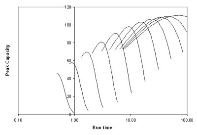 Courtesy Waters Corp
All the treatments above have been general, using analyte plate count as the measure of peak width. However, in gradients, an additional factor plays a role. Due to the difference in solvent composition over its width, the tail of a peak eluting under gradient conditions migrates faster than the front of the peak. As a result, a gradient peak is narrower than the same peak under isocratic conditions in the same solvent composition [1, 7, 8]. This is best demonstrated with step gradients, but the effect is significant for sharp gradients as well.
Peak compression Cg is most pronounced for very sharp gradients. The theory for this relationship has been developed by Poppe and coworkers (9), who derived equation 19:
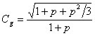 (19)
(19)
The factor p is closely related to the gradient steepness parameter G.
![]() (20)
(20)
As the gradient becomes flat, the peak compression is irrelevant. However, due to the much steeper G for larger molecules, peak compression becomes more pronounced for example in the analysis of peptides. An example of the effect of peak compression is shown in the simulated chromatograms in Figure 6. On the bottom chromatogram you see the peak resolution without compression, on the top you see the improvement due to the compression effect. The analytes are peptides, and the peak compression values were around 0.85, typical for such a sample under real-life conditions. One can see the small but clearly visible improvement in resolution due to peak compression. (Figure 6: simulated chromatograms with (top) and without (bottom) peak compression. )
[1] L. R. Snyder, J. W. Dolan, High-Performance Gradient Elution, The Practical Application of the Linear-Solvent-Strength Model, Wiley-Interscience, Hoboken, New Jersey, 2007
[2] U. D. Neue, Non-linear retention relationships in reversed-phase chromatography, Chromatographia 63 (2006), S45-S53
[3] U. D. Neue, The Theory of Peak Capacity in Gradient Elution, J. Chromatogr. A 1079 (2005), 153-161
[4] U. D. Neue, J. L. Carmody, Y.-F. Cheng, Z. Lu, C. H. Phoebe, and T. E. Wheat, Design of Rapid Gradient Methods for the Analysis of Combinatorial Chemistry Libraries and the Preparation of Pure Compounds, in Advances in Chromatography, Edited by E. Grushka and P. Brown, Vol. 41, 93-136, Marcel Dekker, New York, Basel, 2001
[5] Y.-F. Cheng, Z. Lu, and U. D. Neue, Ultra-Fast LC and LC/MS/MS Analysis, Rapid Commun. Mass Spectrom. 15 (2001), 141-151
[6] J. W. Dolan, L. R. Snyder, N. M. Djordjevic, D. W. Hill and T. J. Waeghe, Reversed-phase liquid chromatographic separation of complex samples by optimizing temperature and gradient time: I. Peak capacity limitations, J. Chromatogr. A 857 (1999), 1-20
[7] L. R. Snyder, D. L. Saunders, J. Chromatogr. Sci. 7 (1969), 195.
[8] U. D. Neue, D. H. Marchand, L. R. Snyder, Peak compression in reversed-phase gradient elution, J. Chromatogr. A 1111 (2006), 32-39
[9] H. Poppe, J. Paanakker, M. Bronckhorst, Peak width in solvent-programmed chromatography, I. General description of peak broadening in solvent-programmed elution, J. Chromatogr. 204 (1981), 77-84


